Description: Train a deep learning model to classify beetles, cockroaches and dragonflies using these images. Note: Original images from https://www.insectimages.org/index.cfm.
Insect Image Dataset
The original dataset is found at the Insect Image websites. There are total 1199 images of beetles, cockroaches and dragonflies. In this project, we will train a neural network model to classfy these three different types of insects. So first let’s take a look at these insects.
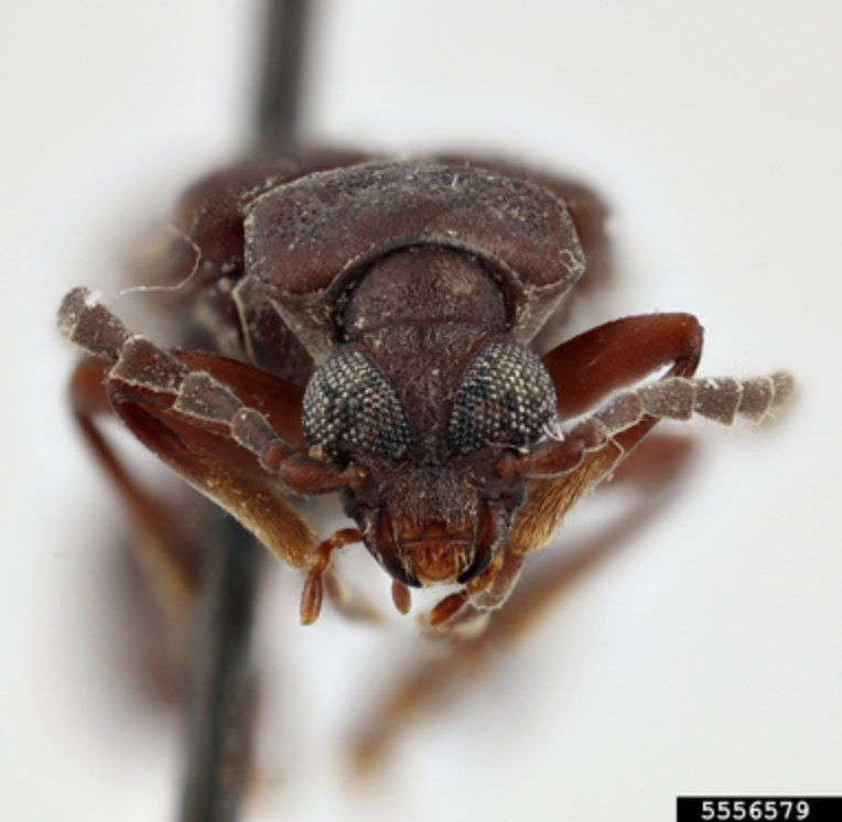
Beetles
import matplotlib.image as mpimg
import matplotlib.pyplot as plt
beetle = mpimg.imread('train/beetles/5556579.jpg')
plt.imshow(beetle)
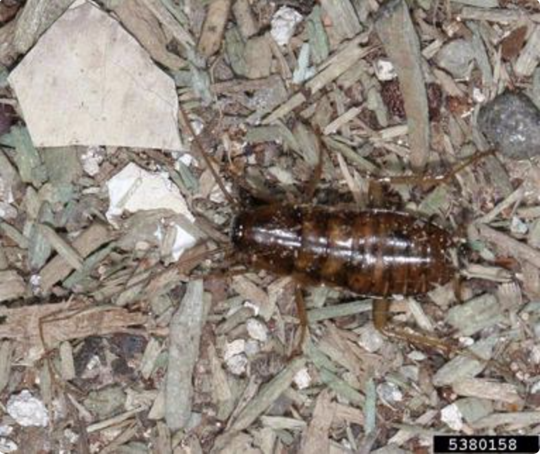
Cockroach
cockroach = mpimg.imread('train/cockroach/5380158.jpg')
plt.imshow(cockroach)
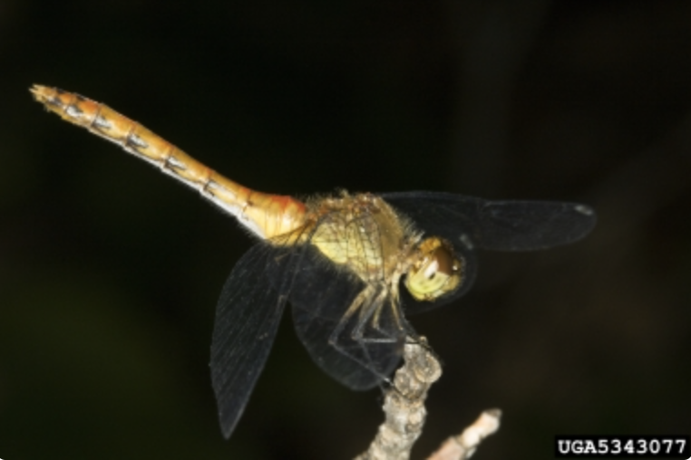
Dragonflies
dragonfly = mpimg.imread('train/dragonflies/5343077.jpg')
plt.imshow(dragonfly)
Load train and test dataset
After we download our train and test dataset, the images may not all consist in the exact same shapes. Thus, we have to resize each image into (64,64,3) (height, width, color channel) shape and stored all images as a numpy array.
def load_images(folder):
    '''load all images in current folder and return as a numpy array
    Parameters
    ----------
    folder: current directory. string

    Return
    ------
    imageArray: array of imgaes. numpy.array

    '''
    images = []
    for filename in os.listdir(folder):
        img = Image.open(os.path.join(folder, filename))
        #img = ImageOps.grayscale(img)
        if img is not None:
            image_resized = img_to_array(img.resize((64, 64)))
            images.append(image_resized)
    return np.array(images)
Now we have 1109 training images and 180 testing images with exact same shape (64,64,3)!
Convolutional Neural network
A Convolutional Neural Network (CNN) is a deep learning algorithm that can recognize and classify features in images for computer vision. It is a multi-layer neural network designed to analyze visual inputs and perform tasks such as image classification, segmentation and object detection.
Build our CNN
Here’s the code:
def ImageModel(input_shape):
    # Define the input placeholder as a tensor with shape input_shape. Think of this as your input image!
    X_input = Input(input_shape)
    X = X_input

    # CONV -> BN -> RELU Block applied to X
    X = Conv2D(32, (4, 4), strides = (1, 1), name = 'conv0')(X)
    X = BatchNormalization(axis = 3, name = 'bn0')(X)
    X = Activation('relu')(X)

    # MAXPOOL
    X = MaxPooling2D((2, 2), name='max_pool1')(X)

    # CONV -> BN -> RELU Block applied to X
    X = Conv2D(64, (4, 4), strides = (1, 1), name = 'conv1')(X)
    X = BatchNormalization(axis = 3, name = 'bn1')(X)
    X = Activation('relu')(X)

    # MAXPOOL
    X = MaxPooling2D((2, 2), name='max_pool2')(X)

    # FLATTEN X (means convert it to a vector) + FULLYCONNECTED
    X = Flatten()(X)
    X = Dense(4, activation='softmax', name='fc')(X)

    # Create model. This creates your Keras model instance, you'll use this instance to train/test the model.
    model = Model(inputs = X_input, outputs = X, name='ImageModel')

    return model
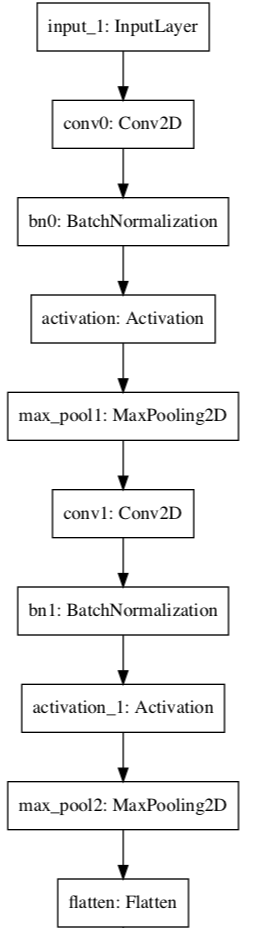
Our CNN network looks like this:
Train
Model.fit(x=X_train, y=y_train, epochs=25, batch_size=64,shuffle=True,verbose=2)
Test
test_loss, test_acc = model.evaluate(X_test, y_test)
test_acc
>>> 0.8111110925674438
The accuracy is about 80%. For a simple model with limited training set, this performance is not bad.
How our model classify insects
To explain how the neural network classified the images, we need to figure out how CNNs work.
How CNNs Works
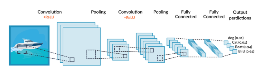
A CNN operates in three stages. The first is a convolution, in which the image is “scanned” a few pixels at a time, and a feature map is created with probabilities that each feature belongs to the required class (in a simple classification example). The second stage is pooling (also called downsampling), which reduces the dimensionality of each feature while maintaining its most important information. The pooling stage creates a “summary” of the most important features in the image.
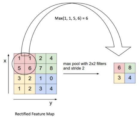
Most CNNs use “max pooling”, in which the highest value is taken from each pixel area scanned by the CNN, as illustrated below.
A CNN can perform several rounds of convolution then pooling. For example, in the first round, an image can be broken down into objects, such as a boat, a person, a plane of grass. In the second round, the CNN can identify features within each object, for example, a face, torso, hands, legs. In a third round, the CNN could go deeper and analyze features within the face, etc.
Finally, when the features are at the right level of granularity, the CNN enters the third stage, which is a fully-connected neural network that analyzes the final probabilities, and decides which class the image belongs to. The final step can also be used for other tasks, such as generating text—a common use of convolutional networks is to automatically generate captions for images.
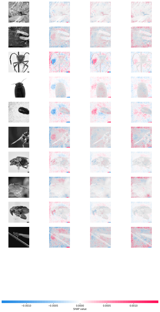
Interpret with SHAP
As we know, SHAP is giving us the opportunity to better understand the model and which features contributed to which prediction. The package allows us to check whether we are taking just features into account which make sense. Thus, machine learning becomes less of a “black box”. This way, we are getting closer to explainable machine learning. The SHAP package is also useful in image recognition tasks.
Here I took the first ten testing insect images as example:
explainer = shap.GradientExplainer(model, X_train)
sv = explainer.shap_values(X_test[:10]);
shap.image_plot([sv[i] for i in range(3)], X_test[:10])