LINEAR SVM
Due Date : 9/28 Monday 10:15 PM EST
import numpy as np
import matplotlib.pyplot as plt
import scipy.io as io
import libsvm
from libsvm.svmutil import *
import pandas as pd

%matplotlib inline
3.1 Linear Support Vector Machine on toy data
3.1.1
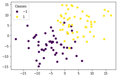
Generate a training set of size $100$ with 2D features (X) drawn at random as follows:
- X_{neg} $\sim$ $\mathcal{N}$($[-5, -5]$, 5*$I_2$) and correspond to negative labels (-1)
- X_{pos} $\sim$ $\mathcal{N}$($[5, 5]$, 5*$I_2$) and correspond to positive labels (+1) Accordingly, $X = [X_{neg}, X_{pos}]$ is a $100\times2$ array, Y is a $100\times1$ array of values $\in {-1, 1}$.
# Generate binary class dataset
np.random.seed(0)

n_samples = 100
center_1 = [-5, -5]
center_2 = [5, 5]
cov = [[25, 0], [0, 25]]

# Generate Data:

Xneg = np.random.multivariate_normal(center_1, cov, (50,1))
Xpos = np.random.multivariate_normal(center_2, cov, (50,1))
X = np.concatenate((Xneg, Xpos), axis=0)
X_x = [each[0][0] for each in X.tolist()]
X_y = [each[0][1] for each in X.tolist()]
Y = 50*[-1]+ 50*[1]

# Scatter plot:
fig, ax = plt.subplots()
scatter = ax.scatter(X_x, X_y, c=Y, label = Y)
legend1 = ax.legend(*scatter.legend_elements(),
                    loc="upper left", title="Classes")
ax.add_artist(legend1)

plt.show()
3.1.2
Train a linear support vector machine on the data with $C=1$ and draw the decision boundary line that separates o and x. Mark the support vectors separately (ex.circle around the point).
Note: You can use the libsvm.svmutil functions with the kernel_type set to 0, indiciating a linear kernel and svm_type set to 0 indicating C-SVC. Also note that the support_vector coefficients returned by the LIBSVM model are the dual coefficients.
# Define the SVM problem

# Define the hyperparameters

# Train the model

# Compute the slope and intercept of the separating line/hyperplanee with the use of the support vectors
# and other information from the LIBSVM model.

# Draw the scatter plot, the decision boundary line, and mark the support vectors.

import svmutil as svm
train = [each[0] for each in X.tolist()]
labels = Y
options = '-s 0 -t 0 -c 1'  # linear model
# Training Model
model = svm.svm_train(labels, train, options)


# Line Parameters
w = np.matmul(np.array(train)[np.array(model.get_sv_indices()) - 1].T, model.get_sv_coef())
b = -model.rho.contents.value
if model.get_labels()[1] == -1:  # No idea here but it should be done :|
    w = -w
    b = -b

print(w)
print(b)

# Plotting
plt.figure(figsize=(6, 6))
for i in model.get_sv_indices():
    plt.scatter(train[i - 1][0], train[i - 1][1], color='red', s=200)
train_ = np.array(train).T
plt.scatter(train_[0], train_[1], c=labels)
plt.plot([-20, 20], [-(-20 * w[0] + b) / w[1], -(20 * w[0] + b) / w[1]])
plt.xlim([-23, 23])
plt.ylim([-23, 23])
plt.show()
[[-0.25088143]
 [-0.21305077]]
-0.017897352332105494
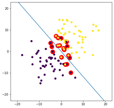
len(model.get_sv_indices())
19
3.1.3
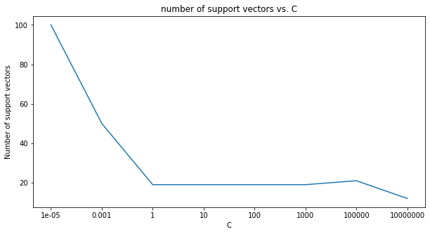
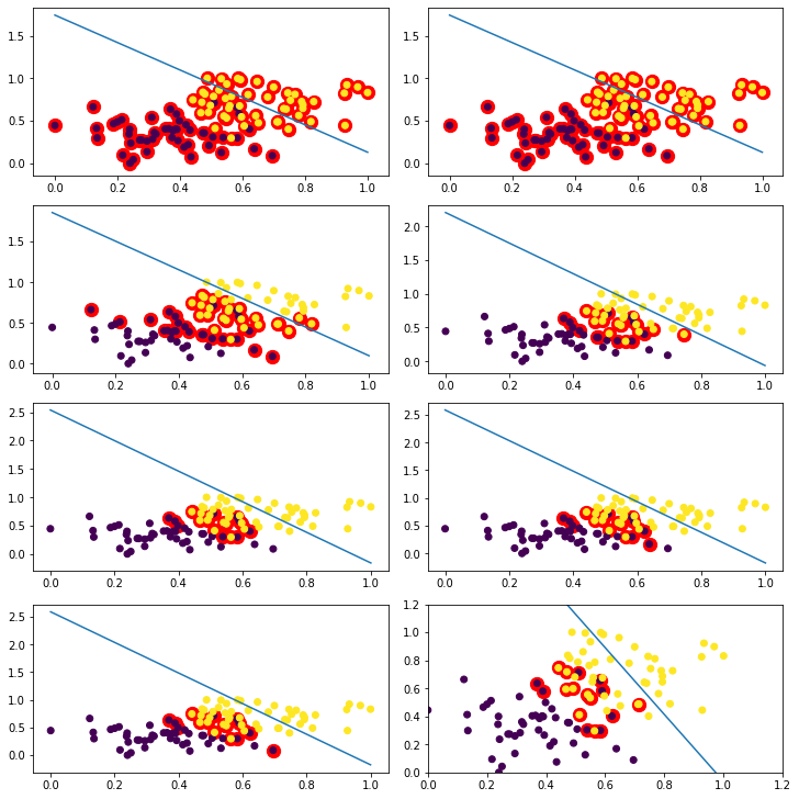
Draw a line that separates the data for 8 different $C$ ($10^{-5}$~$10^7$). Plot the number of support vectors vs. $C$ (plot x-axis on a log scale). How does the number of support vectors change as $C$ increases and why does it change like that?
Note: You might prefer to use the command-line style of svm_parameter initialization such as: svm_parameter('-s 0 -t 0’) to indicate a linear kernel and C-SVC as the SVM type.
C_range = [0.00001, 0.001, 1, 10, 100, 1000, 100000, 10000000]
num_sv = []

# Loop over a similar setup to that in the previous code block.


# Draw the scatter plot with multiple decision lines on top (one for each value of C)

# Draw the num_sv vs. C plot.
fig, ax = plt.subplots(4,2, figsize=(10,10),constrained_layout=True)
x,y = -1,0
for i in range(len(C_range)):

    options = '-s 0 -t 0 -c {}'.format(str(C_range[i]))
    # Training Model
    model = svm.svm_train(labels, train, options)


    # Line Parameters
    w = np.matmul(np.array(train)[np.array(model.get_sv_indices()) - 1].T, model.get_sv_coef())
    b = -model.rho.contents.value
    if model.get_labels()[1] == -1:  # No idea here but it should be done :|
        w = -w
        b = -b

    print(w)
    print(b)

    # Plotting

    if i%2==0:
        y=0
        x+=1
    else:
        y=1
    for i in model.get_sv_indices():
        ax[x,y].scatter(train[i - 1][0], train[i - 1][1], color='red', s=150)
    train_ = np.array(train).T
    ax[x,y].scatter(train_[0], train_[1], c=labels)
    ax[x,y].plot([-20, 20], [-(-20 * w[0] + b) / w[1], -(20 * w[0] + b) / w[1]])
    num_sv.append(len(model.get_sv_indices()))

plt.xlim([-23, 23])
plt.ylim([-23, 23])
plt.show()
[[-0.00491118]
 [-0.00519984]]
0.007284677090644842
[[-0.09364763]
 [-0.10929941]]
0.0601523754299799
[[-0.25088143]
 [-0.21305077]]
-0.017897352332105494
[[-0.25097506]
 [-0.21306215]]
-0.01793960641056622
[[-0.25093309]
 [-0.21310541]]
-0.017922034263428473
[[-0.25119112]
 [-0.21342248]]
-0.01785023293529991
[[-0.27970303]
 [-0.21088177]]
0.2891490144541231
[[-0.5855392 ]
 [ 2.03500762]]
-11.101604764472537
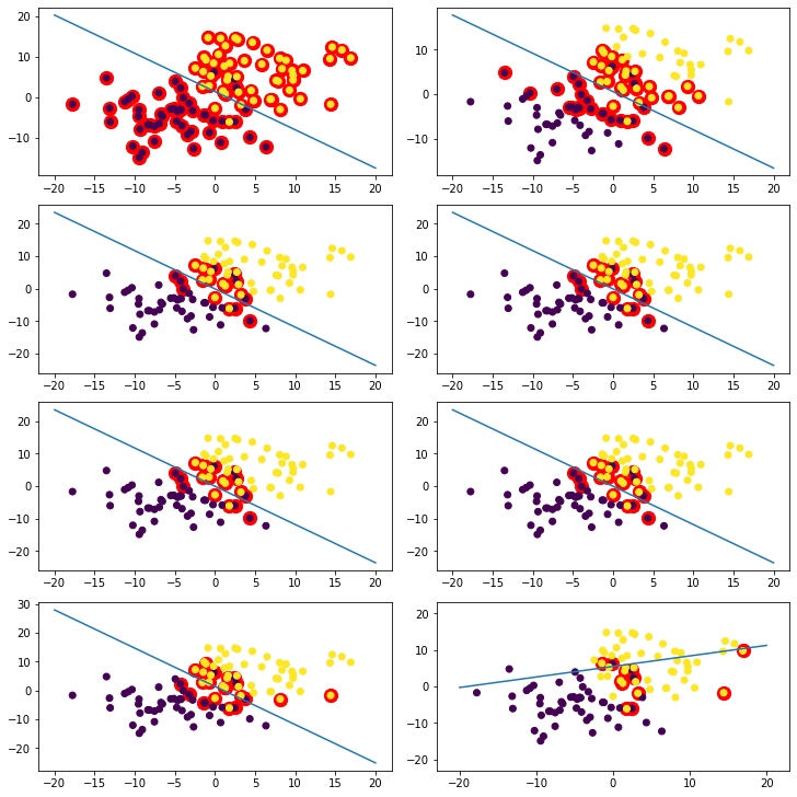
xlabel = [str(each) for each in C_range]
fig, ax = plt.subplots(1,1, figsize=(10,5))
ax.plot(xlabel,num_sv)
ax.set_xlabel('C', fontsize=10)
ax.set_ylabel('Number of support vectors', fontsize=10)
plt.title('number of support vectors vs. C')
Text(0.5, 1.0, 'number of support vectors vs. C')
3.1.4
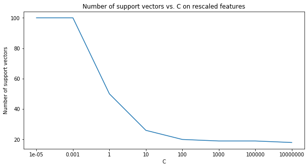
Now try rescaling the data to the $[0,1]$ range and repeat the steps of the previous question (3.1.3) and over the same range of $C$ values. Are the decision boundaries different from those in the previous question? What does this imply about (a) the geometric margin and (b) the relative effect of each feature on the predictions of the trained model ?
Solution below:
SVM tries to maximize the distance between the separating plane and the support vectors. If one feature (i.e. one dimension in this space) has very large values, it will dominate the other features when calculating the distance. If you rescale all features (e.g. to $[0, 1]$), they all have the same influence on the distance metric.
import sklearn
from sklearn import preprocessing
min_max_scaler = preprocessing.MinMaxScaler()

# Single line below:
X_train_minmax = min_max_scaler.fit_transform(train)
C_range = [10**-5, 10**-3, 1, 10, 100, 10**3, 10**5, 10**7]
num_sv = []

# Repeat the loop from 3.1.3
fig, ax = plt.subplots(4,2, figsize=(10,10),constrained_layout=True)
x,y = -1,0
for i in range(len(C_range)):

    options = '-s 0 -t 0 -c {}'.format(str(C_range[i]))
    # Training Model
    model = svm.svm_train(labels, X_train_minmax, options)


    # Line Parameters
    w = np.matmul(np.array(X_train_minmax)[np.array(model.get_sv_indices()) - 1].T, model.get_sv_coef())
    b = -model.rho.contents.value
    if model.get_labels()[1] == -1:  # No idea here but it should be done :|
        w = -w
        b = -b

    print(w)
    print(b)

    # Plotting

    if i%2==0:
        y=0
        x+=1
    else:
        y=1
    for i in model.get_sv_indices():
        ax[x,y].scatter(X_train_minmax[i - 1][0], X_train_minmax[i - 1][1], color='red', s=150)
    X_train_minmax_ = np.array(X_train_minmax).T
    ax[x,y].scatter(X_train_minmax_[0], X_train_minmax_[1], c=labels)
    ax[x,y].plot([0, 1], [-(-1 * w[0] + b) / w[1], -(1 * w[0] + b) / w[1]])
    num_sv.append(len(model.get_sv_indices()))

plt.xlim([0, 1.2])
plt.ylim([0, 1.2])
plt.show()
[[-0.00014161]
 [-0.00017554]]
0.00016433532983978205
[[-0.01416115]
 [-0.01755394]]
0.016433532983996413
[[-3.18780107]
 [-3.62545683]]
3.5383995678022244
[[-6.34642227]
 [-5.59748787]]
5.996391448017262
[[-8.40559713]
 [-6.22605762]]
7.414720805000787
[[-8.69764281]
 [-6.30836861]]
7.611512568994826
[[-8.73492171]
 [-6.32123925]]
7.6371129348525
[[-10.88641763]
 [ -9.1388299 ]]
10.302644583268657
xlabel = [str(each) for each in C_range]
fig, ax = plt.subplots(1,1, figsize=(10,5))
ax.plot(xlabel,num_sv)
ax.set_xlabel('C', fontsize=10)
ax.set_ylabel('Number of support vectors', fontsize=10)
plt.title('Number of support vectors vs. C on rescaled features')
pass
3.2 MNIST
Multiclass kernel SVM. In this problem, we’ll use support vector machines to classify the MNIST data set of handwritten digits.
3.2.1
Load in the MNIST data using from the provided mnist-original.mat file on sakai. First split the data into training and testing by simply taking the first 60k points as training and the rest as testing. Then sample 500 data points for each of the 10 categories (for a total of 5000 training points) from the 60k training photos. These 5k points are now our training set. Finally, sample 500 data points for each of the 10 categories from the 10k testing photos. These 5k points are now our testing set.
Note: For data loading, you might want to use scipy.io.loadmat.
import scipy
import scipy.io as sio
from sklearn.model_selection import train_test_split

MNIST = sio.loadmat('mnist-original.mat')
np.random.seed(0)

X = MNIST['data'].T
y = MNIST['label'][0]
#pd.Series(MNIST['label'][0]).unique()
X_train, X_test, y_train, y_test = train_test_split(X, y, test_size=1/7, random_state=42)
X_train.shape, X_test.shape, y_train.shape, y_test.shape
((60000, 784), (10000, 784), (60000,), (10000,))
y_train = np.reshape(y_train, (-1, 1))
y_test = np.reshape(y_test, (-1, 1))
train_con = np.concatenate((X_train, y_train), axis=1)
array([[0., 0., 0., ..., 0., 0., 3.],
       [0., 0., 0., ..., 0., 0., 5.],
       [0., 0., 0., ..., 0., 0., 3.],
       ...,
       [0., 0., 0., ..., 0., 0., 9.],
       [0., 0., 0., ..., 0., 0., 0.],
       [0., 0., 0., ..., 0., 0., 2.]])
test_con = np.concatenate((X_test, y_test), axis=1)
from random import sample
X_train_all = []
for i in range(10):
    X_one = [each.tolist() for each in train_con if each[-1]==i]
    X_sample = sample(X_one,500)
    for each in X_sample:
        X_train_all.append(each)
X_test_all = []
for i in range(10):
    X_one = [each.tolist() for each in test_con if each[-1]==i]
    X_sample = sample(X_one,500)
    for each in X_sample:
        X_test_all.append(each)
len(X_train_all),len(X_test_all)
(5000, 5000)
y_train = [i[-1] for i in X_train_all]
x_train = [i[:-1] for i in X_train_all]
y_test = [i[-1] for i in X_test_all]
x_test = [i[:-1] for i in X_test_all]
np.unique(y_train, return_counts=True) #ensure each label has 500 examples.
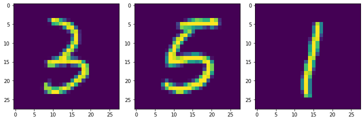
fig, ax = plt.subplots(1,3, figsize=(10,10),constrained_layout=True)
ax[0].imshow(X_train[0].reshape(28,28))
ax[1].imshow(X_train[1].reshape(28,28))
ax[2].imshow(X_train[4].reshape(28,28))
<matplotlib.image.AxesImage at 0x7f9b3b2ebb90>
3.2.3
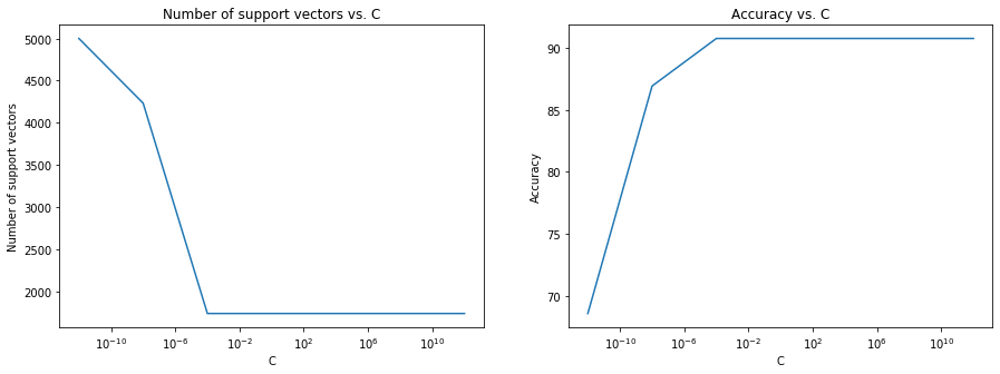
For each value $C=10^{-12}$~$10^{12}$ train a support vector machine with a linear kernel and compute its accuracy on the test set subsampled previously. Plot test accuracy and the number of support vectors (two separate plots) vs. $C$ for $C=10^{-12}$~$10^{12}$ (plot 7 points or more with the x-axis on a log scale).
C_range = [1e-12, 1e-8, 1e-4, 1, 1e4, 1e8, 1e12]

#options = '-s 0 -t 0 -c {}'.format(str(C_range[i]))
    # Training Model
options = '-s 0 -t 0 -c 1'
model = svm.svm_train(y_train, x_train, options)
p_label, p_acc, p_val = svm.svm_predict(y_test, x_test, model)
Accuracy = 90.76% (4538/5000) (classification)
list(p_acc)[0]
90.75999999999999
num_sv = []
p_acc_list = []
for i in range(len(C_range)):

    options = '-s 0 -t 0 -c {}'.format(str(C_range[i]))
    # Training Model
    #options = '-s 0 -t 0 -c 1'
    model = svm.svm_train(y_train, x_train, options)

    p_label, p_acc, p_val = svm.svm_predict(y_test, x_test, model)
    num_sv.append(len(model.get_sv_indices()))
    p_acc_list.append(list(p_acc)[0])
Accuracy = 68.56% (3428/5000) (classification)
Accuracy = 86.92% (4346/5000) (classification)
Accuracy = 90.76% (4538/5000) (classification)
Accuracy = 90.76% (4538/5000) (classification)
Accuracy = 90.76% (4538/5000) (classification)
Accuracy = 90.76% (4538/5000) (classification)
Accuracy = 90.76% (4538/5000) (classification)
p_acc_list
[68.56,
 86.92,
 90.75999999999999,
 90.75999999999999,
 90.75999999999999,
 90.75999999999999,
 90.75999999999999]
num_sv
[5000, 4232, 1734, 1734, 1734, 1734, 1734]
xlabel = C_range
fig, ax = plt.subplots(1,2, figsize=(15,5))
ax[0].plot(xlabel,num_sv)
ax[1].plot(xlabel,p_acc_list)
ax[0].set_xlabel('C', fontsize=10)
ax[0].set_ylabel('Number of support vectors', fontsize=10)
ax[0].set_xscale('log')
ax[0].set_title('Number of support vectors vs. C')
ax[1].set_xlabel('C', fontsize=10)
ax[1].set_ylabel('Accuracy', fontsize=10)
ax[1].set_xscale('log')
ax[1].set_title('Accuracy vs. C')
pass