Instructions
- If there is a conflict bewteen the problem description in the ipython notebook and the question in the pdf, follow the question in the pdf file.
- The part you need to fill in is commented as “Code Clip”. You can search “Code Clip” in this notebook to find the part you need to complete. After you finish the required part, you may need to run other related code blocks for evaluation or visualization.
- If you have a better implementation or find mistakes in this notebook, you could add/modify any function (input, output and return) yourself. Everything is flexible as long as you answered the questions.
import pandas as pd
import numpy as np
import matplotlib.pyplot as plt
import seaborn as sns
from sklearn.model_selection import train_test_split, cross_val_score, KFold
from sklearn.metrics import accuracy_score, auc,roc_curve, roc_auc_score
from sklearn import preprocessing
from sklearn import metrics
from scipy.stats import ttest_ind
Load Training and Testing Data. Get a initial statistics of the training data.
train_data = pd.read_csv('./data_train.csv')
test_data = pd.read_csv('./data_test.csv')
features_mean = list(train_data.columns[1:31])


X_train = train_data.loc[:,features_mean]
y_train = train_data.loc[:, 'diagnosis']

X_test = test_data.loc[:,features_mean]
y_test = test_data.loc[:, 'diagnosis']
3.1 Balanced Dataset
3.1.1 Use 5-fold cross validation on the training set only, and compare accuracy and time cost performance of three different algorithms: ID3, CART and Random Forest,
Code Clip 3.1.1a: Complete the function compare.
from sklearn.metrics import confusion_matrix
def accuracy_per_class(predict, label):
    cm = confusion_matrix(label, predict)
    return np.diag(cm)/np.sum(cm, axis = 1)
import warnings
warnings.filterwarnings("ignore", category=FutureWarning, module="sklearn", lineno=1978)
from sklearn.ensemble import RandomForestClassifier
from sklearn.ensemble import ExtraTreesClassifier
from sklearn.tree import DecisionTreeClassifier
from sklearn.model_selection import KFold
import time
from statistics import mean, stdev
from scipy import stats
#start = time.time()

def compare(X_train, y_train, X_test, y_test, class_weight = None, max_depth = None):

    #accuracy_all = []
    #accuracy_per_class_all = []
    #cvs_all = []
    accuracy_rf = []
    accuracy_cart = []
    accuracy_id3 = []
    time_rf = []
    time_cart = []
    time_id3 = []

    X = np.concatenate([X_train, X_test], axis= 0)
    y = np.concatenate([y_train, y_test], axis= 0)

    # Code Clip 3.1.1a
    #-------------Forest-------------
    # start = time.time()
    # Step 1: Build a random forest and fit the input data.
    # Step 2: Do prediction on the testing set.
    # end = time.time()
    # Step 3: Calculte different metrics: accuracy over testing set,
    #             corss validation score over the whole training set,
    #             accuracy of each class.

    kf = KFold(n_splits=5,shuffle=False)
    #kf.split(train_data)
    for train_index, test_index in kf.split(train_data):
        # Split train-test
        X_cv_train, X_cv_test = X_train.iloc[train_index], X_train.iloc[test_index]
        y_cv_train, y_cv_test = y_train.iloc[train_index], y_train.iloc[test_index]

        start = time.time()
        random_forest = RandomForestClassifier(n_estimators = 60, criterion = "gini")
        random_forest.fit(X_cv_train, y_cv_train)
        pred = random_forest.predict(X_cv_test)
        end = time.time()

        time_rf.append(end-start)
        accuracy_rf.append(accuracy_score(y_cv_test,pred))
        #accuracy_per_class_all.append(accuracy_per_class(pred, y_cv_test))
        #cvs_all.append(cross_val_score(random_forest, X_train, y_train, cv = kf))
        #-------------Split by GINI-------------
        start = time.time()
        cart = DecisionTreeClassifier(criterion = "gini")
        cart.fit(X_cv_train, y_cv_train)
        pred = cart.predict(X_cv_test)
        end = time.time()

        time_cart.append(end-start)
        #accuracy_per_class(pred, y_test)
        accuracy_cart.append(accuracy_score(y_cv_test,pred))
        #accuracy_per_class_all.append(accuracy_per_class(pred, y_cv_test))
        #cvs_all.append(cross_val_score(random_forest, X_train, y_train))

        #-------------Split by Entropy-------------
        start = time.time()
        id3 = DecisionTreeClassifier(criterion = "entropy")
        id3.fit(X_cv_train, y_cv_train)
        pred = id3.predict(X_cv_test)
        end = time.time()
        #accuracy_per_class(pred, y_test)

        time_id3.append(end-start)
        accuracy_id3.append(accuracy_score(y_cv_test,pred))
        #accuracy_per_class_all.append(accuracy_per_class(pred, y_cv_test))
        #cvs_all.append(cross_val_score(random_forest, X_train, y_train))

    return accuracy_rf, accuracy_cart, accuracy_id3, time_rf, time_cart, time_id3
accuracy_rf, accuracy_cart, accuracy_id3, time_rf, time_cart, time_id3 = compare(X_train, y_train, X_test, y_test)
    avg_acc_rf,avg_acc_cart,avg_acc_id3 = mean(accuracy_rf),mean(accuracy_cart),mean(accuracy_id3)
    avg_time_rf,avg_time_cart,avg_time_id3 = mean(time_rf),mean(time_cart),mean(time_id3)
    std_acc_rf,std_acc_cart,std_acc_id3 = stdev(accuracy_rf),stdev(accuracy_cart),stdev(accuracy_id3)
Code Clip 3.1.1b: Do pairwise t-tests to determine whether there’s a significant difference between the best algorithm and the other algorithms. (Hint: You could first use sklearn.model_selection.KFold to get 5 different train/val division on the training set.)
# Code Clip 3.1.1b
stats.ttest_rel(accuracy_rf,accuracy_cart)
Ttest_relResult(statistic=1.6417788607745119, pvalue=0.1759802114476083)
stats.ttest_rel(accuracy_rf,accuracy_id3)
Ttest_relResult(statistic=1.1876701108169152, pvalue=0.3006678235482861)
stats.ttest_rel(accuracy_id3,accuracy_cart)
Ttest_relResult(statistic=1.5136732103419446, pvalue=0.20466711250685823)
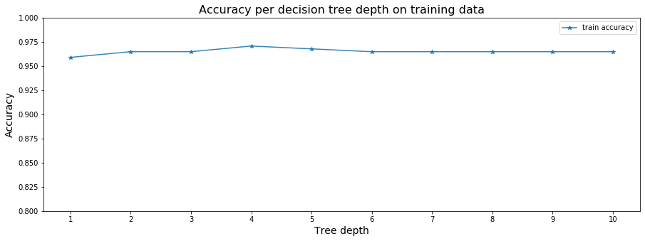
3.1.2 Effect of the depth.
Code Clip 3.1.2: Complete the function run_cross_validation_on_trees.
def run_cross_validation_on_trees(X, y, tree_depths, cv=5, scoring='accuracy'):
#     cv_scores_list = []
#     cv_scores_std = []
#     cv_scores_mean = []
     accuracy_scores = []

#     for depth in tree_depths:
        # Get the accuracy,  mean, std of the cross validation score.

     for depth in tree_depths:
        accuracy_rf = []
        kf = KFold(n_splits=cv,shuffle=False)
        #kf.split(train_data)
        for train_index, test_index in kf.split(train_data):
            # Split train-test
            X_cv_train, X_cv_test = X_train.iloc[train_index], X_train.iloc[test_index]
            y_cv_train, y_cv_test = y_train.iloc[train_index], y_train.iloc[test_index]

            random_forest = RandomForestClassifier(n_estimators=60,max_depth = depth,min_samples_split=2,random_state = 0)
            random_forest.fit(X_cv_train, y_cv_train)
            pred = random_forest.predict(X_cv_test)

            accuracy_rf.append(accuracy_score(y_cv_test,pred))

        accuracy_scores.append(mean(accuracy_rf))
    # return what you need
#     return cv_scores_mean, cv_scores_std, accuracy_scores
     return accuracy_scores

# function for plotting cross-validation results
def plot_cross_validation_on_trees(depths, accuracy_scores, title):
    fig, ax = plt.subplots(1,1, figsize=(15,5))
    #ax.plot(depths, cv_scores_mean, '-o', label='mean cross-validation accuracy', alpha=0.9)
    #ax.fill_between(depths, cv_scores_mean-2*cv_scores_std, cv_scores_mean+2*cv_scores_std, alpha=0.2)
    #ylim = plt.ylim()
    ax.plot(depths, accuracy_scores, '-*', label='train accuracy', alpha=0.9)
    ax.set_title(title, fontsize=16)
    ax.set_xlabel('Tree depth', fontsize=14)
    ax.set_ylabel('Accuracy', fontsize=14)
    ax.set_ylim([0.8,1])
    ax.set_xticks(depths)
    ax.legend()
sm_tree_depths = range(1,11)
# get what you returned.
sm_accuracy_scores = run_cross_validation_on_trees(X_train, y_train, sm_tree_depths)
print(sm_accuracy_scores)


# plotting accuracy
plot_cross_validation_on_trees(sm_tree_depths, sm_accuracy_scores,
                               'Accuracy per decision tree depth on training data')
plt.show()

# Play: Only uses the first ten features.
# sm_cv_scores_mean2, sm_cv_scores_std2, sm_accuracy_scores2 = run_cross_validation_on_trees(X_train.iloc[:,:10],
#                                                                                         y_train, sm_tree_depths)

# # plotting accuracy
# plot_cross_validation_on_trees(sm_tree_depths, sm_cv_scores_mean2, sm_cv_scores_std2, sm_accuracy_scores2,
#                                'Accuracy per decision tree depth on training data')
# plt.show()
[0.9590366581415175, 0.964919011082694, 0.964919011082694, 0.9707587382779199, 0.9678175618073316, 0.9648763853367434, 0.9648763853367434, 0.9648763853367434, 0.9648763853367434, 0.9648763853367434]
random_forest = RandomForestClassifier(n_estimators=60,max_depth = 4,min_samples_split=2,random_state = 0)
pred = random_forest.fit(X_train, y_train).predict(X_test)
accuracy = accuracy_score(y_test,pred)
accuracy
0.9534883720930233
3.1.3 ROC and vairable importance
Code Clip 3.1.3a: Complete the function draw_roc_with_feature_idx. Then finished the next two steps (AUC of different features and Draw ROC Curve of the first five features.
def plot_roc(fpr, tpr, roc_auc, title = ''):
    plt.figure()
    lw = 2
    plt.plot(fpr, tpr, color='darkorange',
             lw=lw, label='ROC curve (area ={})'.format(roc_auc))
    plt.plot([0, 1], [0, 1], color='navy', lw=lw, linestyle='--')
    plt.xlim([0.0, 1.0])
    plt.ylim([0.0, 1.05])
    plt.xlabel('False Positive Rate')
    plt.ylabel('True Positive Rate')
    plt.title('Receiver operating characteristic over {}'.format(title))
    plt.legend(loc="lower right")
    plt.show()


def draw_roc_with_feature_idx(X_test, y_test, i, draw = False):

    # Code Clip 3.1.3
    # calculate list of false positive rate and true positive rate.
    # calculate AUC.

    #if draw:
    #    plot_roc(fpr, tpr, roc_auc, title = 'Feature' + str(i))

    return 0#auc
fpr_all = []
tpr_all = []
AUC_all = []
for i in range(30):
    y_score = X_train.iloc[:,i].copy()
    fpr, tpr, thresholds = roc_curve(y_train, y_score)
    fpr_all.append(fpr)
    tpr_all.append(tpr)
    AUC_all.append(auc(fpr, tpr))

fig, ax = plt.subplots(3,2, figsize=(10,10),constrained_layout=True)
for i in range(5):
        ax[0,0].plot(fpr_all[i],tpr_all[i], '--', label='Feature'+str(i+1), alpha=0.9)
        ax[0,0].set_xlabel('False Positive Rate', fontsize=14)
        ax[0,0].set_ylabel('True Positive Rate', fontsize=14)
ax[0,0].legend()
for i in range(5,10):
        ax[0,1].plot(fpr_all[i],tpr_all[i], '--', label='Feature'+str(i+1), alpha=0.9)
        ax[0,1].set_xlabel('False Positive Rate', fontsize=14)
        ax[0,1].set_ylabel('True Positive Rate', fontsize=14)
ax[0,1].legend()
for i in range(10,15):
        ax[1,0].plot(fpr_all[i],tpr_all[i], '--', label='Feature'+str(i+1), alpha=0.9)
        ax[1,0].set_xlabel('False Positive Rate', fontsize=14)
        ax[1,0].set_ylabel('True Positive Rate', fontsize=14)
for i in range(15,20):
        ax[1,1].plot(fpr_all[i],tpr_all[i], '--', label='Feature'+str(i+1), alpha=0.9)
        ax[1,1].set_xlabel('False Positive Rate', fontsize=14)
        ax[1,1].set_ylabel('True Positive Rate', fontsize=14)
for i in range(20,25):
        ax[2,0].plot(fpr_all[i],tpr_all[i], '--', label='Feature'+str(i+1), alpha=0.9)
        ax[2,0].set_xlabel('False Positive Rate', fontsize=14)
        ax[2,0].set_ylabel('True Positive Rate', fontsize=14)
for i in range(25,30):
        ax[2,1].plot(fpr_all[i],tpr_all[i], '--', label='Feature'+str(i+1), alpha=0.9)
        ax[2,1].set_xlabel('False Positive Rate', fontsize=14)
        ax[2,1].set_ylabel('True Positive Rate', fontsize=14)
ax[1,0].legend()
ax[1,1].legend()
ax[2,0].legend()
ax[2,1].legend()
<matplotlib.legend.Legend at 0x7fe66a2b4190>
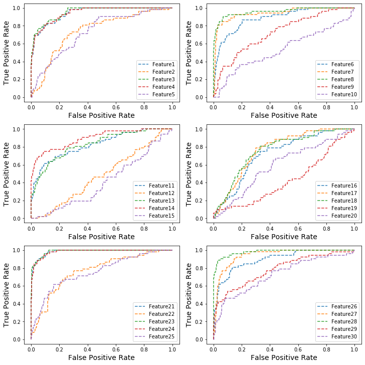
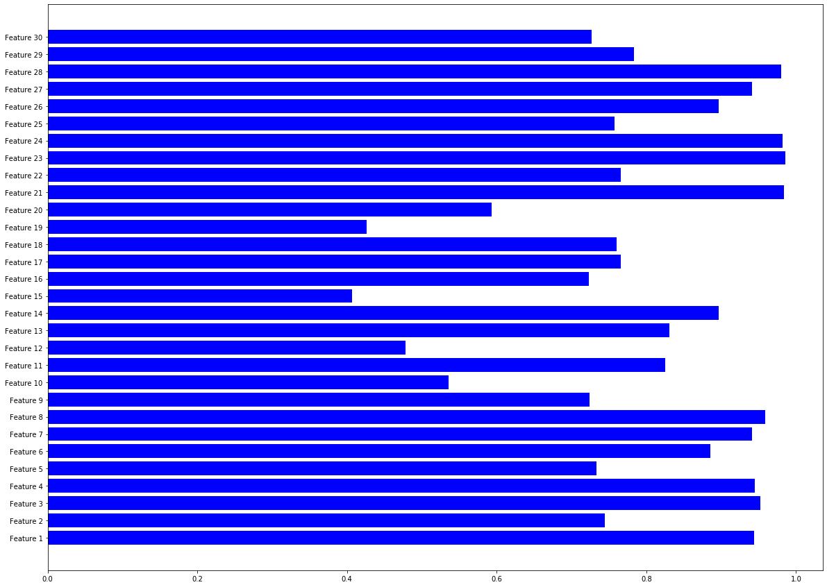
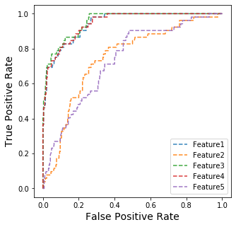
Do you think some features might be more useful than others?
Ans: Some features like feature 8,21,23,24,28 might be more useful than others because their AUC are larger than others.
AUC of different features
Code clip 3.1.3b, You may find plt.bar useful here.
plt.figure(figsize=(20,15))

name_list = []
# Code Clip 3.1.3b
for i in range(30):
    name_list.append("Feature "+str(i+1))


plt.barh(range(len(AUC_all)), AUC_all,color='b',tick_label=name_list)
plt.show()
#plt.xlabel('Feature Number')
#plt.ylabel('AUC')
#plt.title('AUC of different features')
#plt.legend(loc="lower right")
#plt.show()
Draw ROC Curve of the first five features
fig, ax = plt.subplots(1,1, figsize=(5,5))
for i in range(5):
        ax.plot(fpr_all[i],tpr_all[i], '--', label='Feature'+str(i+1), alpha=0.9)
        ax.set_xlabel('False Positive Rate', fontsize=14)
        ax.set_ylabel('True Positive Rate', fontsize=14)
ax.legend()
<matplotlib.legend.Legend at 0x7fe667856ed0>
3.1.4 Partial ROC
Code Clip 3.1.4 Follow the intruction in the question. You could test the correctness of your code by setting $t_0 = 0, t_1= 1$.
# Code Clip 3.1.4
for i in range(5):
    feature = np.array(X_train.iloc[:,i])
    partial_roc_auc = roc_auc_score(y_train,feature,max_fpr = 0.2)
    print("Feature "+ str(i) + "'s partial auc: " +str(partial_roc_auc))
Feature 0's partial auc: 0.8642425582080755
Feature 1's partial auc: 0.5964117300324197
Feature 2's partial auc: 0.8800839964633068
Feature 3's partial auc: 0.8669134983790157
Feature 4's partial auc: 0.6059902740937224
3.1.5 Model Reliance of CART model
Code Clip 3.1.5 Follow the instruction in the question.
# Code Clip 3.1.5
cart = DecisionTreeClassifier(criterion = "gini")
cart.fit(X_train, y_train)
pred = cart.predict(X_train)
accuracy_CART = accuracy_score(y_train,pred)
#print(accuracy_CART)
#print(X_train)
#type(X_train)
for i in range(X_train.shape[1]):
    copy = X_train.copy()
    copy.iloc[:,i] = np.random.permutation(copy.iloc[:,i].values)
    #print(copy)
    pred_scramble = cart.predict(copy)
    accuracy_feature = accuracy_score(y_train,pred_scramble)
    #print(accuracy_feature)
    loss = 100*(accuracy_CART-accuracy_feature)/accuracy_CART
    print("Feature "+str(i+1)+" gets loss: "+("%.3f" % loss)+'%')
Feature 1 gets loss: 4.094%
Feature 2 gets loss: 0.000%
Feature 3 gets loss: 0.000%
Feature 4 gets loss: 0.000%
Feature 5 gets loss: 0.000%
Feature 6 gets loss: 0.000%
Feature 7 gets loss: 0.000%
Feature 8 gets loss: 0.000%
Feature 9 gets loss: 0.000%
Feature 10 gets loss: 0.000%
Feature 11 gets loss: 0.000%
Feature 12 gets loss: 0.000%
Feature 13 gets loss: 0.000%
Feature 14 gets loss: 0.000%
Feature 15 gets loss: 0.585%
Feature 16 gets loss: 0.000%
Feature 17 gets loss: 1.462%
Feature 18 gets loss: 0.000%
Feature 19 gets loss: 0.000%
Feature 20 gets loss: 0.877%
Feature 21 gets loss: 14.620%
Feature 22 gets loss: 0.000%
Feature 23 gets loss: 3.216%
Feature 24 gets loss: 0.000%
Feature 25 gets loss: 0.000%
Feature 26 gets loss: 0.000%
Feature 27 gets loss: 0.000%
Feature 28 gets loss: 19.591%
Feature 29 gets loss: 0.000%
Feature 30 gets loss: 0.000%
3.2 Imbalanced Dataset
train_data = pd.read_csv('./data_imbalanced_train.csv')
test_data = pd.read_csv('./data_imbalanced_test.csv')

features_mean = list(train_data.columns[1:31])

X_train = train_data.loc[:,features_mean]
y_train = train_data.loc[:, 'diagnosis']

X_test = test_data.loc[:,features_mean]
y_test = test_data.loc[:, 'diagnosis']
3.2.1: What is the ratio between the two labels ?
Code Clip 3.2.1
# Code Clip 3.2.1

positive = len([i for i in y_train if i==1])
negative = len([i for i in y_train if i==0])
if positive>negative:
    imbalance_ratio = negative/positive
    print("Class 0 is less common class.")
else:
    imbalance_ratio = positive/negative
    print("Class 1 is less common class.")

imbalance_ratio
Class 1 is less common class.


0.1793103448275862
3.2.2 Use three algorithms from Problem 3.1 to train models on the training set. Please report the confusion matrix on the test set.
Code Clip 3.2.2
# Code Clip 3.2.2

random_forest = RandomForestClassifier(n_estimators = 60, criterion = "gini")
pred_rf = random_forest.fit(X_train, y_train).predict(X_test)
cm_rf = confusion_matrix(y_test,pred_rf)

cart = DecisionTreeClassifier(criterion = "gini")
cart.fit(X_train, y_train)
pred_cart = cart.predict(X_test)
cm_cart = confusion_matrix(y_test,pred_cart)

id3 = DecisionTreeClassifier(criterion = "entropy")
id3.fit(X_train, y_train)
pred_id3 = id3.predict(X_test)
cm_id3 = confusion_matrix(y_test,pred_id3)
cm_rf, cm_cart, cm_id3
(array([[66,  1],
        [ 2, 17]]), array([[63,  4],
        [ 4, 15]]), array([[65,  2],
        [ 2, 17]]))
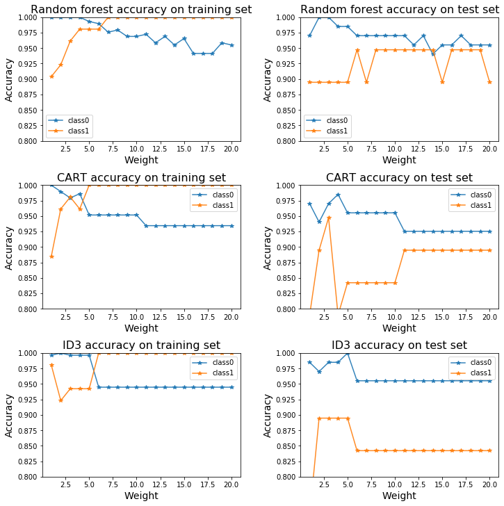
3.2.3 For each class, get the accuracy on the training set and testing set with different sample reweighting parameters. Plot them according to the reweight parameter. (Set the maximum depth of all the algorithms to 3).
Code Clip 3.2.3:
weight_list = list(np.arange(1, 21))

rf_acc_train = []
rf_acc_test = []
cart_acc_train = []
cart_acc_test = []
id3_acc_train = []
id3_acc_test = []

for weight in weight_list:
    # Code Clip 3.2.3
    # Calculte the accuracy of each class.
    class_weight = {0: 1.,
                1: weight}


    random_forest = RandomForestClassifier(n_estimators = 60, max_depth = 3, criterion = "gini", class_weight=class_weight)
    random_forest.fit(X_train, y_train)
    pred_rf_train = random_forest.predict(X_train)
    pred_rf_test = random_forest.predict(X_test)
    rf_acc_train.append(accuracy_per_class(pred_rf_train, y_train))
    rf_acc_test.append(accuracy_per_class(pred_rf_test, y_test))

    cart = DecisionTreeClassifier(criterion = "gini", max_depth = 3, class_weight = class_weight)
    cart.fit(X_train, y_train)
    pred_cart_train = cart.predict(X_train)
    pred_cart_test = cart.predict(X_test)
    cart_acc_train.append(accuracy_per_class(pred_cart_train, y_train))
    cart_acc_test.append(accuracy_per_class(pred_cart_test, y_test))

    id3 = DecisionTreeClassifier(criterion = "entropy", max_depth = 3, class_weight=class_weight)
    id3.fit(X_train, y_train)
    pred_id3_train = id3.predict(X_train)
    pred_id3_test = id3.predict(X_test)
    id3_acc_train.append(accuracy_per_class(pred_id3_train, y_train))
    id3_acc_test.append(accuracy_per_class(pred_id3_test, y_test))
cart_acc_train
[array([1.        , 0.88461538]),
 array([0.98965517, 0.96153846]),
 array([0.97931034, 0.98076923]),
 array([0.9862069 , 0.96153846]),
 array([0.95172414, 1.        ]),
 array([0.95172414, 1.        ]),
 array([0.95172414, 1.        ]),
 array([0.95172414, 1.        ]),
 array([0.95172414, 1.        ]),
 array([0.95172414, 1.        ]),
 array([0.93448276, 1.        ]),
 array([0.93448276, 1.        ]),
 array([0.93448276, 1.        ]),
 array([0.93448276, 1.        ]),
 array([0.93448276, 1.        ]),
 array([0.93448276, 1.        ]),
 array([0.93448276, 1.        ]),
 array([0.93448276, 1.        ]),
 array([0.93448276, 1.        ]),
 array([0.93448276, 1.        ])]
[each[0] for each in cart_acc_train]
[1.0,
 0.9896551724137931,
 0.9793103448275862,
 0.9862068965517241,
 0.9517241379310345,
 0.9517241379310345,
 0.9517241379310345,
 0.9517241379310345,
 0.9517241379310345,
 0.9517241379310345,
 0.9344827586206896,
 0.9344827586206896,
 0.9344827586206896,
 0.9344827586206896,
 0.9344827586206896,
 0.9344827586206896,
 0.9344827586206896,
 0.9344827586206896,
 0.9344827586206896,
 0.9344827586206896]
fig, ax = plt.subplots(3,2, figsize=(10,10), constrained_layout=True)
#ax.plot(depths, cv_scores_mean, '-o', label='mean cross-validation accuracy', alpha=0.9)
#ax.fill_between(depths, cv_scores_mean-2*cv_scores_std, cv_scores_mean+2*cv_scores_std, alpha=0.2)
#ylim = plt.ylim()
rf_acc_train_class0 = [each[0] for each in rf_acc_train]
rf_acc_train_class1 = [each[1] for each in rf_acc_train]
rf_acc_test_class0 = [each[0] for each in rf_acc_test]
rf_acc_test_class1 = [each[1] for each in rf_acc_test]

cart_acc_train_class0 = [each[0] for each in cart_acc_train]
cart_acc_train_class1 = [each[1] for each in cart_acc_train]
cart_acc_test_class0 = [each[0] for each in cart_acc_test]
cart_acc_test_class1 = [each[1] for each in cart_acc_test]

id3_acc_train_class0 = [each[0] for each in id3_acc_train]
id3_acc_train_class1 = [each[1] for each in id3_acc_train]
id3_acc_test_class0 = [each[0] for each in id3_acc_test]
id3_acc_test_class1 = [each[1] for each in id3_acc_test]

ax[0,0].plot(weight_list, rf_acc_train_class0, '-*', label='class0', alpha=0.9)
ax[0,0].plot(weight_list, rf_acc_train_class1, '-*', label='class1', alpha=0.9)
ax[0,0].set_title('Random forest accuracy on training set', fontsize=16)
ax[0,0].set_xlabel('Weight', fontsize=14)
ax[0,0].set_ylabel('Accuracy', fontsize=14)
ax[0,0].set_ylim([0.8,1])
ax[0,0].legend()

ax[0,1].plot(weight_list, rf_acc_test_class0, '-*', label='class0', alpha=0.9)
ax[0,1].plot(weight_list, rf_acc_test_class1, '-*', label='class1', alpha=0.9)
ax[0,1].set_title('Random forest accuracy on test set', fontsize=16)
ax[0,1].set_xlabel('Weight', fontsize=14)
ax[0,1].set_ylabel('Accuracy', fontsize=14)
ax[0,1].set_ylim([0.8,1])
ax[0,1].legend()

ax[1,0].plot(weight_list, cart_acc_train_class0, '-*', label='class0', alpha=0.9)
ax[1,0].plot(weight_list, cart_acc_train_class1, '-*', label='class1', alpha=0.9)
ax[1,0].set_title('CART accuracy on training set', fontsize=16)
ax[1,0].set_xlabel('Weight', fontsize=14)
ax[1,0].set_ylabel('Accuracy', fontsize=14)
ax[1,0].set_ylim([0.8,1])
ax[1,0].legend()

ax[1,1].plot(weight_list, cart_acc_test_class0, '-*', label='class0', alpha=0.9)
ax[1,1].plot(weight_list, cart_acc_test_class1, '-*', label='class1', alpha=0.9)
ax[1,1].set_title('CART accuracy on test set', fontsize=16)
ax[1,1].set_xlabel('Weight', fontsize=14)
ax[1,1].set_ylabel('Accuracy', fontsize=14)
ax[1,1].set_ylim([0.8,1])
ax[1,1].legend()

ax[2,0].plot(weight_list, id3_acc_train_class0, '-*', label='class0', alpha=0.9)
ax[2,0].plot(weight_list, id3_acc_train_class1, '-*', label='class1', alpha=0.9)
ax[2,0].set_title('ID3 accuracy on training set', fontsize=16)
ax[2,0].set_xlabel('Weight', fontsize=14)
ax[2,0].set_ylabel('Accuracy', fontsize=14)
ax[2,0].set_ylim([0.8,1])
ax[2,0].legend()

ax[2,1].plot(weight_list, id3_acc_test_class0, '-*', label='class0', alpha=0.9)
ax[2,1].plot(weight_list, id3_acc_test_class1, '-*', label='class1', alpha=0.9)
ax[2,1].set_title('ID3 accuracy on test set', fontsize=16)
ax[2,1].set_xlabel('Weight', fontsize=14)
ax[2,1].set_ylabel('Accuracy', fontsize=14)
ax[2,1].set_ylim([0.8,1])
ax[2,1].legend()

plt.show()